During this series, we will use Tenyks to build a Data-Centric pipeline to debug and fix a model trained with the NVIDIA TAO Toolkit.
Part 1. We demystify the NVIDIA ecosystem and define a Data-Centric pipeline based on a model trained with the NVIDIA TAO framework.
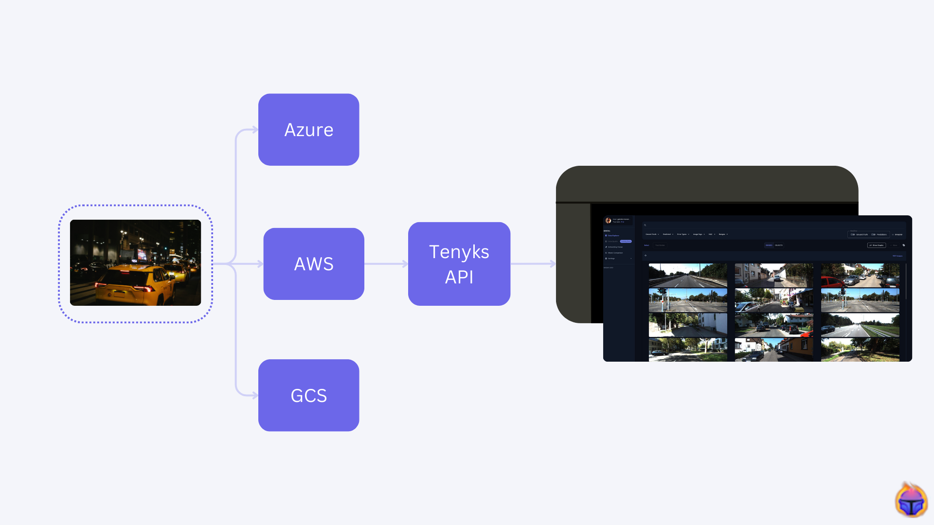
Part 2. Using the Tenyks API, we show you how to upload a dataset and a model to the Tenyks platform.
Part 3 (current). We identify failures in our model due to data issues, fix these failures and improve our model’s performance with the fixed dataset.
💡Don’t miss our previous series on NVIDIA TAO Toolkit: tips and tricks, & model comparison.
Table of Contents
- Recap from Part 2
- Finding model failures
- Improving performance by fixing a dataset
- Conclusion
1. Recap from Part 2
In the second post of this series we focused on two main things:
- We set up a data storage provider.
- We established a workflow to ingest our data into the Tenyks platform using the Tenyks API.
Before continuing, make sure that you have the following:
- A dataset and a model on your Tenyks account (see Figure 1)

2. Finding model failures
2.1 mAP Analysis
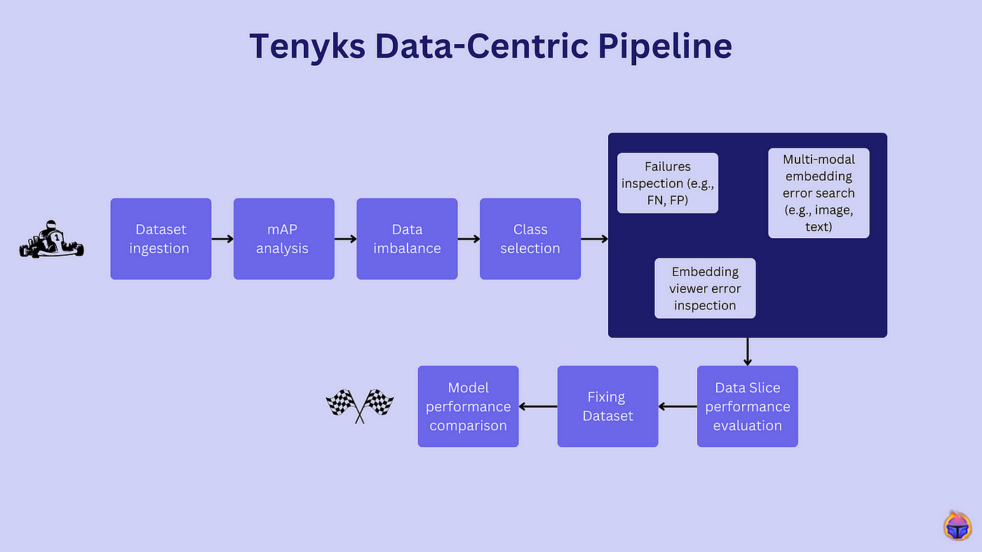
In the first stage of our Data-Centric pipeline we ingested our dataset (see Figure 2). Now, let’s focus on the next stage: mAP analysis.
💡For a refresher on mean average precision (mAP), visit our article on mAP, where we carefully explain how this metric is computed and demystify a few misunderstandings around it.
Figure 3. Mean average precision (mAP) of the crosswalks class
On the Tenyks dashboard, we select Model Comparison on the left menu. From there we can quickly obtain a picture of the per-class performance as shown on Figure 3.
The very first insight we obtain from this view is the poor performance of the “crosswalks” class:
- The “crosswalks” class has the lowest performance: ~0.26 mAP.
- The “crosswalks” class has the lowest recall: ~0.40 mAR.
- Out of 154 annotations for the “crosswalks” class, the model is predicting 170 objects in total.
Based on these findings, we can start to make some hypotheses 👩🔬:
- The model has both a precision and a recall problem: it erroneously predicts a high number of “crosswalks” objects, and it fails to detect many ground truth “crosswalks” objects.
- This model behaviour could be attributed to some of the following issues: label quality, edge cases, or mispredictions, among others.
2.2 Data imbalance
Now, to evaluate data imbalance issues, let’s first verify the distribution of our annotations and our predictions.
Figure 4. Frequency of annotations and predictions
- As reflected on Figure 4, the dataset, in general, is imbalanced. For instance, the “vehicles” class contains 10 times more annotations than the “bicycles” class.
- Despite the imbalance, the class with the lowest number of annotations (i.e., “bicycles” class) performs better than the “crosswalks” class.
- The “crosswalks” class is on par with the “motorcycles” class in number of annotations, yet the performance of the former is considerably lower: out of 154 “crosswalks” objects, the model is wrongly predicting the majority of them.
🤔 Can we simply add more samples of the “crosswalks” class to balance our data? The answer is NO. We need to add the right kind of “crosswalks” examples (or we risk obtaining the same performance). Before identifying the kind of samples we need, we must find why our model is failing to predict and to detect this class.
💡Hint: We often see an imbalance issue and believe that the first thing we need to do is to apply data augmentation techniques. But, contrary to popular belief, this is often the wrong approach. We show one example of this scenario on this Roboflow article.
2.3 Class selection
Once we have run the previous two stages of our Data-Centric pipeline, we can see with more clarity where and how to start:
- We will fix the “croswalks” class because it has the widest room for improvement in performance (i.e., 80/20 rule: a successful yet tiny improvement can yield the highest reward).
- We can analyze the False Negative and the False Positive examples to make some hypotheses of what is wrong with our “croswalks” class.
- We will search for label quality issues reflected in errors such as mispredictons or mislabelled examples.
Now, imagine we have built our own mAP and mAR tooling, or let’s say we are using W&B to plot precision-recall curves. We might have arrived to similar conclusions as in Section 3.1, and 3.2 but now, how can we find the root causes of our data issues?
2.4 Failure inspection
Figure 5. Multi-Class confusion matrix for object detection
Tenyks multi-class confusion matrix provides us with a summary of errors such as False Negative, False Positive and Mispredictions.
On Figure 5, we observe the following:
- 84 “croswalks” objects are undetected (i.e., false negatives).
- 107 “croswalks” objects are incorrectly predicted (i.e., false positives).
- 6 “croswalks” objects are misprediected.
- 63 “croswalks” objects are true positives.
Let’s analyze the false negative examples using the Data Explorer:
Figure 6. Analyzing undetected objects in our dataset
Figure 6 provides key insights on the type of undetected objects where the model is failing:
- Samples with fading crosswalks.
- Crosswalks that are in a diagonal position.
- Crosswalks that are behind other objects (i.e., occlusion).
2.5 Using multi-modal search to find similar errors
Next, let’s double down on the fading crosswalks as one of the potential data issues!
Figure 7. Using text search to retrieve “fading crosswalks”
On Figure 7, we use a combination of error filters and text search to retrieve similar examples. These retrieved examples are grouped in a Data Slice (see Section 2.6 for more details).
We can observe that many of the retrieved examples are in fact undetected objects.
Our model is failing at detecting fading crosswalks, but the interesting questions is now: How can we quantify how bad our model is failing due to the fading crosswalks?
Let’s use Tenyks Data Slices to answer the above question!
2.6 Tenyks Data Slices: evaluate performance on a subset of our data
After forming one potential hypothesis of why our model is failing, we will evaluate our model on the Data Slice of images containing fading crosswalks.
A Data Slice is a group of samples from our dataset that share some common characteristics. They are often used to evaluate how a model performs on that particular set of images.
Figure 8. Evaluating performance on a Data Slice containing “fading crosswalks” examples
Figure 8 illustrates how we can use Tenyks Model Comparison to compare:
- Our model performance on the “crosswalks” class in general.
- Our model performance on a data slice containing samples with faded “crosswalks”.
As shown on Figure 8, the model performance on the faded “crosswalks” dropped by more than half the amount of our baseline. Hence, we have found one of the root causes of our low model performance on the “crosswalks” class 🎊.
Is this the only cause of low performance? 🤔
2.7 Other causes of low model performance
A rapid second look at the dataset using the Data Explorer shows that our data suffers from label quality issues.\
Figure 9. Other potential causes of poor model performance
Figure 9 illustrates a few examples of the following issues:
- Missing annotations: objects that are in fact “crosswalks” that weren’t labelled.
- Mislabelled examples: objects that were assigned a “crosswalks” label, when they are not.
3. Improving performance by fixing the dataset
To improve performance, we will focus our efforts on two main tasks:
- Fixing the faded “crosswalks” issue by adding more examples of faded “crosswalks” to our dataset
- Fixing the missing annotations and the mislabelled examples in the “crosswalks” class
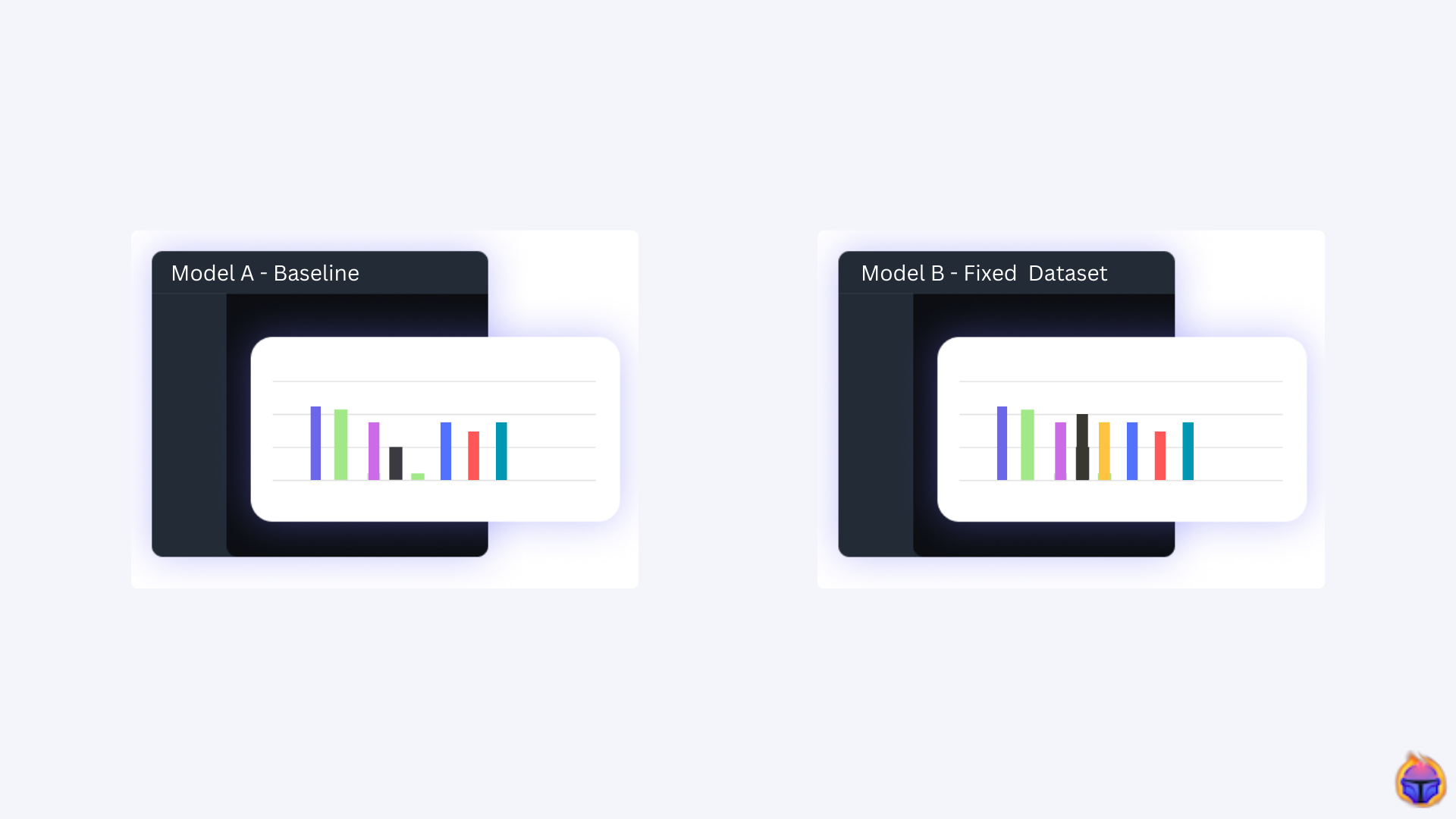
Figure 10. Left side: Baseline model, Right side: Model with fixed dataset
For the sake of brevity we don’t illustrate the whole process to address (1) and (2). Instead Figure 10 demonstrates that after fixing the data issues, and generating a new dataset (that can be downloaded here), the performance for the “crosswalks” class improved from 0.27 mAP to 0.81 mAP, and from 0.40 mAR to 0.87 mAR 🚀.
4. Conclusion
Our goal for this Series was twofold. First, we sought to identify errors, failures, and biases within a dataset that could lead to poor model performance. Second, once these data failures were pinpointed, our goal was to rectify these errors, ultimately training a model with improved performance.
In this last leg, Part 3, following our Data-Centric pipeline, we defined a specific low performing class to fix, the “crosswalks” class. Then, we systematically identified the reasons behind the low performance leveraging Tenyks ML tools for data debugging. After using Tenyks embedding search we created a Data Slice containing faded “crosswalks” samples, which were actually the main root cause of the low performance.
After fixing the dataset, we were able to improve model performance in our “crosswalks” class from ~0.27 mAP to ~0.81 mAP.
If you’re all-in, as we are, on the future of Computer Vision, don’t miss our article Computer Vision Pipeline 2.0, where we argue how Foundation Models are bringing a new paradigm in the applied Computer Vision landscape.
Authors: Jose Gabriel Islas Montero, Dmitry Kazhdan.
If you would like to know more about Tenyks, sign up for a sandbox account.